LSH – an efficient approach to nearest neighbour search

In Image similarity search with LIRE we explained how to compare and find similar images using the Java library LIRE. The idea was to transform the complicated problem of comparing a large bunch of pixels to the simpler problem of comparing vectors representing histograms and other higher-level properties. In other words, if we can compress the information inherent in a bunch of pixels to a point in n-dimensional space (an array with n entries – the so called feature vector of the image), we can regard the distance between two such points as a similarity measure for the corresponding images. We can then find the images similar to a search image by selecting those images whose feature vectors have a small distance to the feature vector of the search image.

However, a naive approach to the problem – comparing the feature vector of the search image to all feature vectors in the database – is rather slow if our database is large. In this article, we show how to implement a fast similarity search for even very large databases.

The basic idea

To avoid comparing thousands of n-dimensional vectors in every lookup we employed a hashing technique which maps similar vectors to the same buckets in a hash table. Thus, finding similar images in even very large databases reduces to calculating a single hash and considering all the images in the same bucket. In what follows, we present this technique called Locality Sensitive Hashing (LSH) and our implementation of it in some detail.

The concept resembles other well-known problems in computer science. For example, hash tables can be employed to look up whether some string is in a huge set of strings. You simply put all the strings in the set into a hash table. After that, determining whether a search string is in the set reduces to calculating the hash of the search string and checking whether the search string is in the bucket for this hash. This is much faster than comparing the search string to all strings in the database.

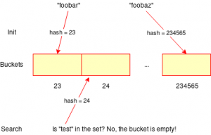
However, this method will not normally put similar strings in the same buckets in the hash table. For example, „foobar“ might end up at position 23 in the hash table, whereas „foobaz“ might end up at position 234565. The crucial additional idea of LSH is to find a hash function that gives guarantees that it is very likely that similar keys are mapped to the same buckets (or nearby buckets; however, we ignore this complication in this article).

… and images?

To apply the idea to images, we need to „hash“ them. This is done in a two-step process. First we apply so-called feature extraction – a process to retrieve information from the source and represent it in a vector space. This is basically what libraries like LIRE do. Second, we calculate the hash of the feature vector. The additional magic happens in the second step: we use a hashing method mapping similar feature vectors to similar bucket indices.

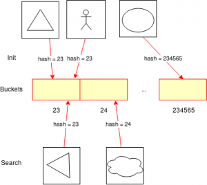
To be sure, with this technique it is neither guaranteed that all images in the same bucket are similar nor that all similar images are in the same bucket. What can be shown, however, is that the applied hashing techniques provide certain probabilities for matches. It is likely that we find similar images in the same bucket, but we still have to do the full comparison with the images in the bucket determined by the hash. In the example on the left, for example, the rotated triangle is identified as having a similar match in the database (the other triangle), but the bucket also contains the image of a person. Merely comparing all feature vectors in the same bucket is still faster than comparing all feature vectors in the database.

Being „locality-sensitive“

A common and effective method to hash feature vectors by similarity is the so-called Random Projection Method. It creates a hash table index using a formula like this:

$$(p \circ \lfloor{(\frac{1}{q}\cdot (v \cdot W + e)}\rfloor)\mod{s}$$

The central idea is that the weights \(W\), the projection vector \(p\), and the offset values \(e\) are selected at random for each hash table. In fact, since \(W\) is a matrix, it represents a whole bunch of random weightings of the different components of the input vector. Multiplying \(W\) with the feature vector \(v\) yields a vector of weighted sums. These sums are modified by adding the vector \(e\). By taking the dot product with \(p\) (which yields a scalar value), we get an algorithm that overall maps similar input vectors to similar indices.

As to the other components of the formula:

• \(\lfloor \cdot \rfloor\) is the floor operator which has to be read component-wise.
• \(s\) is the size of the hash table.
• \(\frac{1}{q}\) is simply a scaling factor, called the bucket size. It has to be determined by experiment. As a rule of thumb, the greater \(q\) is, the more images end up in the same bucket. Thus, the multiplication has to be read component-wise.

LSH Implementation

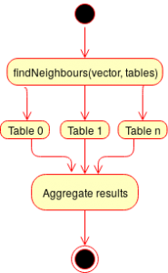We worked hard to make our implementation very flexible and customizable to support as much use-cases as possible. Writing a simple tool which implements the formula and connects it with LIRE is fairly simple. However it was mandatory to use a whole bunch of tables with different individual parameters. This is why we introduced a Table-layer. Each table manages its own configuration such as a different size or error correction values. Thanks to this layer it is also possible for us to combine several tables with different feature vectors.

There are a few more implementation details worth mentioning:

• False-positive detection: when having a very limited amount of hash tables it is possible that some sources land in the same bucket despite their differences. When reducing complex data into a simple hash it is always possible that equal results point to entirely different sources. To solve this easily we introduced a simple API to re-check all results from a given bucket using distance algorithms such as the Euclidean Distance. Before returning the results computed by LSH to a client it is possible to filter all results. However this feature enables further applications: in some cases a user should be able to decide how „similar“ the search results should be. In such a case all values from a given bucket can be re-checked using this API to drop not close enough neighbours.
• Mapping tables: the tables described above will be stored in a Redis database which keeps all of its values in memory for fast lookups and allows syncing to disk to reduce the risk of a possible data loss. Internally each table will be represented by a hash table which associates a bucket index with a list of UUIDs pointing to the similar sources. As each hash table is represented by a UUID as key, several tables for several applications of LSH can be used simultaneously without a big effort. However this part of LSH is abstracted by a storage contract to not force anyone to use Redis.
  
• Providing metadata: our current implementation only cares about the UUIDs of an extracted source in the end. This separation from metadata such as product descriptions or URLs has been done intentionally to avoid any limitations caused by assuming a special metadata layout. Our exemplary implementati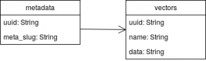on stores the data computed by LSH in a Redis database and persists additional metadata about the source such as descriptions in an SQL database. On the right is a simple diagram which shows the data structure. It provides a metadata table which contains a UUIDv5 to uniquely identify the source by its raw data to avoid storing the same image twice and a slug which contains a json-encoded string with all the metadata. Through a one-to-many relation this is associated to a vectors table. It contains all extracted features from libraries like LIRE to avoid re-extractions for sources when using multiple tables with the same features, but different hash parameters. Additionally the feature vectors can be used for the optional false-positive checks. This structure provides the information about the sources that can be exposed via an API. However it is completely optional and not a part of LSH itself, so it is possible to omit this feature and connect our LSH module to any sort of existing data source assuming that the existing structure can be linked to the UUID generated by our module.

Conclusion

The main task of LSH is to replace the complex per-component comparisons with a simple lookup in a hash table which results in a noticeable performance improvement. Furthermore LSH can be used as a general-purpose technique which means that it can be adopted for any vector-based nearest-neighbour search. Besides libraries such as LIRE there are tools like Facenet for images with faces or Strugatzki for sound extraction from songs that can be used with our LSH implementation to detect similarities in such sources. Thanks to the ability to compose several features it is even possible to define a chain of extractors to compare complex sources according to multiple criteria.

Our project has been implemented in Scala using Akka. During the process we learned a lot about the development and deployment with Docker and the setup of pipelines for continuous integration and delivery with GitLab CI. In order to share the things we’ve learned, more articles about the technology we’ve used are planned for the future.